Accuracy evaluation

Measuring the accuracy of point forecasts

Let’s look at the M3 yearly data. In our exploratory analysis we used the prediction-realization diagram to assess the distribution of actuals and forecasts. We spotted some zero actuals and negative forecasts, which makes some popular metrics such as MAPE difficult to use. But even having only positive actuals and forecasts, MAPE can be unreliable or even misleading (Davydenko and Fildes, 2013). Nonetheless, MAPE remains very popular. So let’s see how to calculate it (even though there are better options).

First, let’s load the data (if we haven’t done it yet)

library(forvision)
# load time series actuals
ts <- m3_yearly_ts
# load forecasts
fc <- m3_yearly_fc

Now let’s look at how many cases contain non-positive actuals or forecasts:

# create a dataframe containing both actuals and forecasts formatted using the AFTS format 
af <- createAFTS(ts, fc)
# find the percentage of "bad" cases
nrow(subset(af, value <=0 | forecast <=0)) / nrow(af) * 100

## 0.1515152

The percentage of “bad” cases is negligible (<1%), so let’s exclude them and proceed to obtaining the accuracy table and chart for MAPE:

# exclude bad cases
af2 <- subset(af, value > 0 & forecast > 0)
# calculate MAPEs
calculateMAPEs(af2)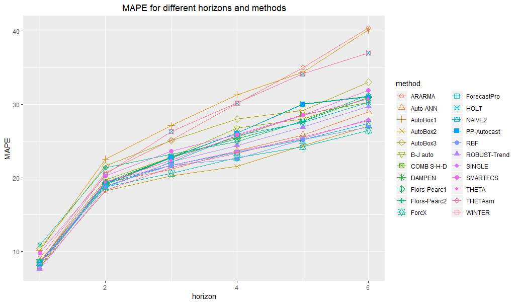

To overcome the problems of MAPE, we can use MASE (Hyndman and Koehler, 2006) instead:

# calculate MASEs
calculateMASEs(ts, af)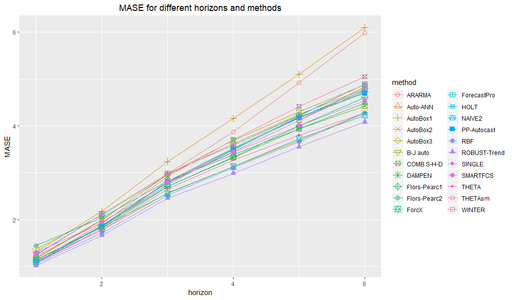

For the M3 data we have only fixed-origin forecasts. But in case of rolling-origin forecasts we can use AvgRelMAE instead, as it has some advantages such as being less affected by outliers and more indicative of relative performance under linear loss (Davydenko and Fildes, 2013).

Assessing the adequacy of prediction intervals

The above tools were designed to measure the accuracy of point forecasts. But we may also want try to assess the adequacy of interval predictions. To do this, we need to use the plotCoverage() function.

Let’s use our example where we calculated prediction intervals for ARIMA and ETS using the forecast package

# load data
ts <- m3_quarterly_ts
fc <- m3_quarterly_fc_pis
# create a dataframe containing both actuals and forecasts formatted using the AFTS format 
af <- createAFTS(ts, fc)
# show coverage chart for ETS forecast method
plotCoverage(af, "ETS", pi = 90)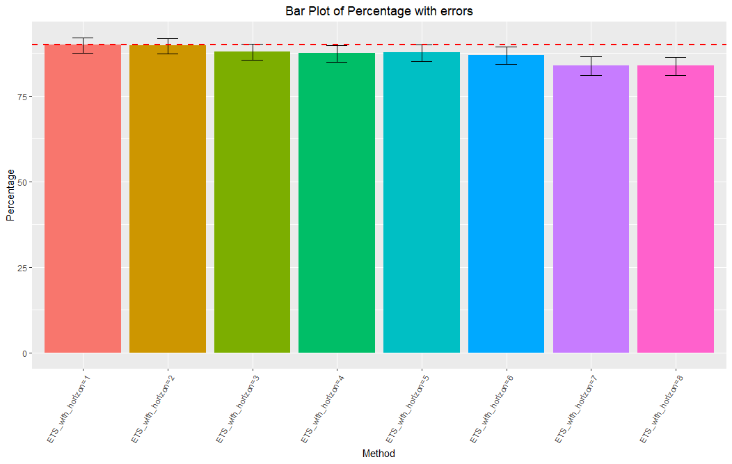

# show coverage chart for ARIMA forecast method
plotCoverage(af, "ARIMA", pi = 90)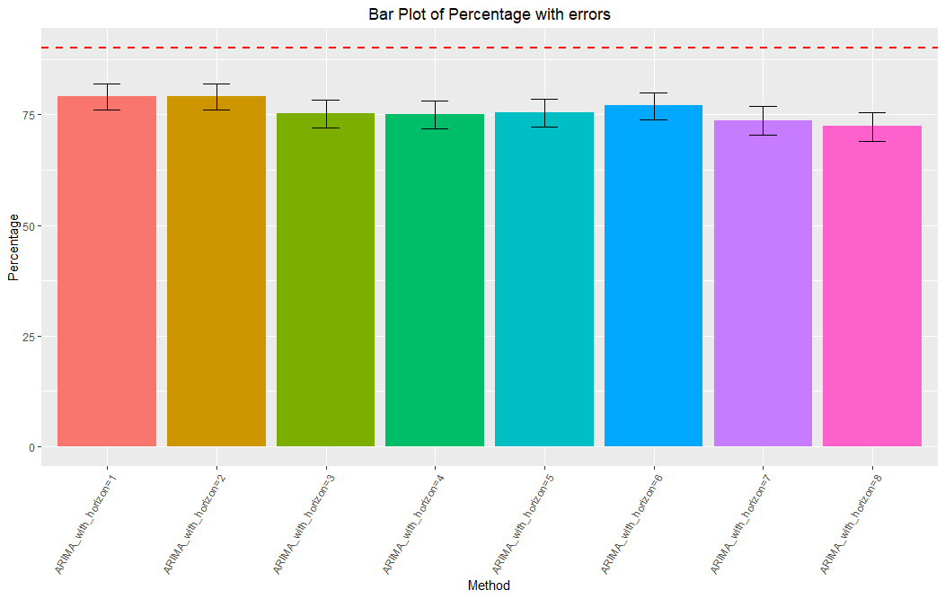

By looking at the coverage chart, it can be seen that the auto.arima method tends to underestimate the uncertainty associated with the forecasts produced, whereas the ets method gives more adequate results.

References:

Davydenko, Andrey & Robert Fildes. (2013). Measuring Forecasting Accuracy: The Case of Judgmental Adjustments to Sku-Level Demand Forecasts. International Journal of Forecasting 29 (3). Elsevier B.V.: 510–22. doi:10.1016/j.ijforecast.2012.09.002.

Hyndman, R.J. and Koehler, A.B. (2006). Another look at measures of forecast accuracy. International Journal of Forecasting, 22(4), 679-688.

To cite this website, please use the following reference:

Sai, C., Davydenko, A., & Shcherbakov, M. (date). The Forvision Project. Retrieved from https://forvis.github.io/

_{© 2018 Sai, C., Davydenko, A., & Shcherbakov, M. All Rights Reserved. Short sections of text, not exceed two paragraphs, may be quoted without explicit permission, provided that full acknowledgement is given.}