Navigation :

Exploratory analysis

After loading input data, need to explore it in order to

double-check if the data was loaded and prepared correctly
examine the range and the distribution for forecasts and actuals
detect possible outliers or unexpected cases, the presence of zero cases, negative cases, missing actuals and the frequency of such cases

Eventually, at this step we want i) to confirm that the data is of appropriate quality for measuring accuracy performance and ii) to choose the error metrics that correspond to the features of the data.

To explore the distribution of actuals and forecasts, let’s use the prediction-realization diagram.

# load yearly M3-data
# load time series actuals
library(forvision)
ts <- m3_yearly_ts
# load forecasts
fс <- m3_yearly_fc

# create a dataframe containing both actuals and forecasts formatted using the AFTS format 
library(forvision)
af <- createAFTS(ts, fc)

# plot the prediction-realization diagram
plotPRD(af)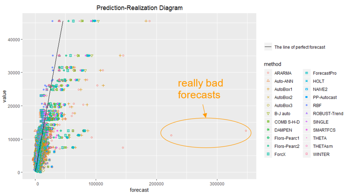

The graph spots some really unwanted cases when forecast seriously overestimated actuals. E.g., having a forecast close to 350,000 units we had actual of only about 11,000 units. We also observe negative forecasts while actuals are always non-negative.

Let’s take a closer look at the “really bad forecasts” spotted. With the AFTS format we can slice-and-dice forecast data in order to find the details:

subset(af, forecast > 100000)

##       series_id category    value timestamp   method_id forecast horizon origin_timestamp
## 14862      Y113    MICRO  7475.00      1992    ARARMA 144595.0       4             1988
## 14884      Y113    MICRO 11160.00      1993    ARARMA 224119.6       5             1988
## 14906      Y113    MICRO 12505.00      1994    ARARMA 347381.2       6             1988
## 43810      Y332  FINANCE 26099.16      1993  AutoBox1 112117.0       6             1987
## 43814      Y332  FINANCE 26099.16      1993    ARARMA 102439.7       6             1987
## 44030      Y334  FINANCE 30636.26      1991  AutoBox1 107644.4       4             1987
## 44034      Y334  FINANCE 30636.26      1991    ARARMA 111450.1       4             1987
## 44052      Y334  FINANCE 35104.84      1992  AutoBox1 140253.9       5             1987
## 44056      Y334  FINANCE 35104.84      1992    ARARMA 144957.9       5             1987
## 44073      Y334  FINANCE 45525.66      1993  B-J auto 103875.3       6             1987
## 44074      Y334  FINANCE 45525.66      1993  AutoBox1 182804.6       6             1987
## 44078      Y334  FINANCE 45525.66      1993    ARARMA 188824.7       6             1987

For series_id=’Y113’ one of the actuals is 7475.00, while the corresponding forecast is 144595.0 – a huge forecast error. Let’s show this forecast on the graph.

First, in order visualization tools to work correctly, we must prepare appropriate time-based object timestamp columns for the data_ts and data_fs:

library(zoo)
ts$timestamp_dbo <- as.yearmon(ts$timestamp, format = '%Y')
fc$timestamp_dbo <- as.yearmon(fc$timestamp, format = '%Y')

Then we can show forecasts produced at origin=1988 using a set of methods (say, “ARARMA”, “HOLT”, “NAIVE2”) using the fixed origin graph:

plotFixedOrigin(ts, fc, "Y113",  1988, c("ARARMA", "HOLT", "NAIVE2"))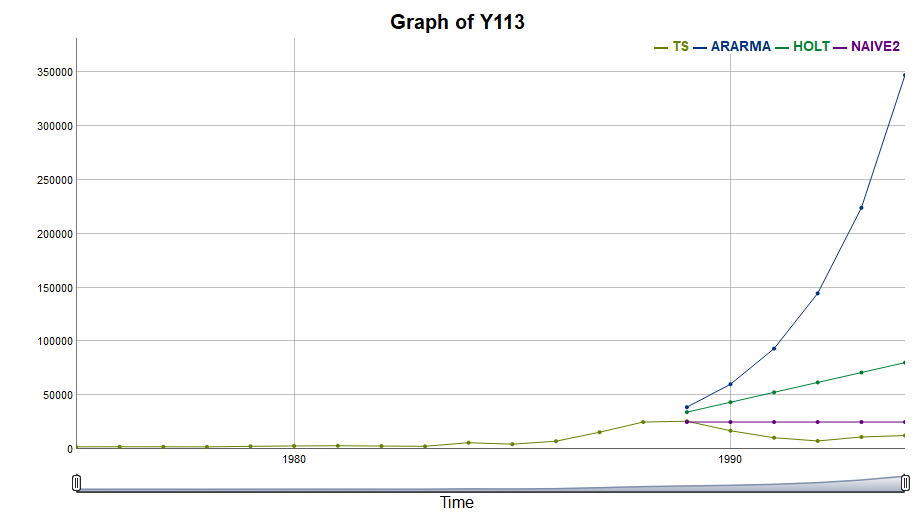

Method “ARARMA” are performing quite badly since it tend to extrapolate trends that do not hold in subsequent periods. Thus, the prediction-realization diagram together with the fixed origin graph helped identify the risks associated with using some methods like “ARARMA”. However, it’s just how the forecast methods works like, so there are no unexpected cases here.

When working with interval predictions, we may want to visualize the forecast uncertainty using the fan chart.

# load quarterly M3-data
# load time series actuals
ts <- m3_quarterly_ts
# load forecasts
fc <- m3_quarterly_fc_pis

# prepare appropriate time-based object timestamp columns for the data_ts and data_fs
library(zoo)
ts$timestamp_dbo <- as.yearqtr(ts$timestamp, format = '%Y-Q%q')
fc$timestamp_dbo <- as.yearqtr(fc$timestamp, '%Y-Q%q')

# plot a fan chart
plotFanChart(ts, fc,  "Q1", "1992-Q4", "ARIMA")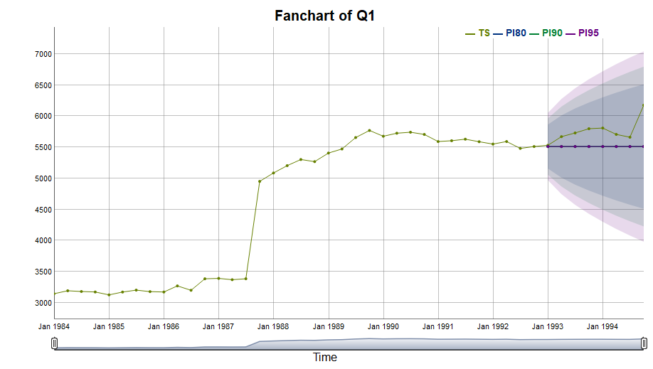

After visual exploration of the input data and confirming that it is of appropriate quality, we can proceed to applying formal techniques to measure forecasting performance and compare alternative forecasting techniques.

To cite this website, please use the following reference:

Sai, C., Davydenko, A., & Shcherbakov, M. (date). The Forvision Project. Retrieved from https://forvis.github.io/

_{© 2018 Sai, C., Davydenko, A., & Shcherbakov, M. All Rights Reserved. Short sections of text, not exceed two paragraphs, may be quoted without explicit permission, provided that full acknowledgement is given.}